(2005-07-22)
The Former Problem with Electromagnetic Units
A science which hesitates to forget its founders is lost.
Alfred North
Whitehead
(1861-1947)
This section is of historical interest only, you are advised to
skip it
if you were blessed with an education entirely grounded
on Giorgi's electrodynamic units (SI units based on the MKSA system).
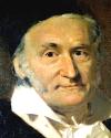
The first consistent system of mechanical units was the
meter-gram-second system advocated by Carl Friedrich Gauss in 1832.
It was used by Gauss and Weber (c.1850)
in the first definitions of electromagnetic units in absolute terms.
However, the term Gaussian system now refers to a particular
mix of electrical C.G.S. units (discussed below) once dominant
in theoretical investigations.
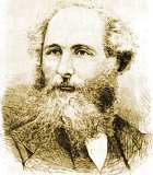
James Clerk Maxwell himself was instrumental in bringing about the
cgs system in 1874 (centimeter-gram-second).
Two sets of electrical units were made part of the system.
An enduring confusion results from the fact that the quantities measured by these
different units have different definitions
(in modern terms, for example,
the magnetic quantity now denoted B could be either B or cB).
Following Maxwells own vocabulary, it's customary to speak of either
electrostatic units (esu) or
electromagnetic units (emu).
Originally, none of the C.G.S. electromagnetic units had specific names.
On August 25th, 1900, the
International
Electrical Congress adopted two names :
- Gauss for the C.G.S. unit of magnetic field:
1 G = 10 -4 T.
- Maxwell for the C.G.S. unit of magnetic flux:
1 Mx = 10 -8 Wb.
The maxwell, still known as a line of force,
is called abweber (abWb)
using the later naming of CGS electrical units after their
MKSA counterparts. Likewise, the gauss
(1 maxwell per square centimeter)
is also called abtesla (abT).
For electrostatic CGS units (esu)
the prefix stat- is used instead...
Electrodynamic units are now based on a proper independent electrical unit,
as advocated by the Italian engineer Giovanni Giorgi (1871-1950) in 1901:
The addition of the ampère to the MKS system has turned it
into a consistent 4-dimensional system (MKSA)
which is the foundation for modern SI units.

Scholars from bygone days should be credited
for accomplishing so much in spite of such confusing systems.
(2005-07-15)
The Lorentz Force
The Lorentz force on a test particle defines
the electromagnetic field(s).
The expression of the Lorentz force introduced here defines dynamically the fields
which are governed by Maxwell's equations,
as presented further down.
Neither of these two statements is a logical consequence of the other.
We offer no apology for our resolutely anachronistic presentation:
The concept of an electric field is due to Michael Faraday (1791-1867) while
the modern expression of the force exerted by an electromagnetic field on a moving
electric charge is due to H.A. Lorentz (1853-1928).
In electrostatics, the electric field E
present at the location of a particle of charge q
summarizes the influence of all other electric charges, by stating that
the particle is submitted to an electrostatic force equal to q E.
This defines E.
This concept may be extended to
magnetostatics for a moving test particle.
More generally, the electromagnetic fields need not be
constant in the following expression of the force acting on a particle of charge
q moving at velocity v.
The average force exerted per unit of volume may thus be expressed in terms of
the density of charge r
and the density of current j.
(2005-07-18)
Electrostatics:
On the electric field from static charges.
Coulomb's inverse square law
translates into the local differential property of the field expressed by Gauss,
namely: div E = r/eo
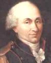
 The SI unit of electric charge is named after the French military engineer
Charles
Augustin de Coulomb (1736-1806). Using a torsion balance,
Coulomb discovered, in 1785, that the electrostatic force between two charged particles is proportional
to each charge, and inversely proportional to the square of the distance
between them.
In modern terms, Coulomb's Law reads:
The SI unit of electric charge is named after the French military engineer
Charles
Augustin de Coulomb (1736-1806). Using a torsion balance,
Coulomb discovered, in 1785, that the electrostatic force between two charged particles is proportional
to each charge, and inversely proportional to the square of the distance
between them.
In modern terms, Coulomb's Law reads:
Electrostatic Force
between Two Charged Particles
| || F || = |
| q q' | |
 |
| 4peo r 2 |
| |
The direction of the electrostatic force
is on the line joining the two charges.
The force is repulsive
between charges of the same sign (both negative or both positive).
It's attractive between charges of unlike signs.
In the language of fields introduced above,
all of the above is summarized by the following
expression, which gives the electrostatic field E
produced at position r by a motionless particle of charge q
located at the origin:
Electrostatic Field of a Point Charge at the Origin
| E = |
q r |
|
| 4peo r 3 |
| |
Since r / r 3
is the opposite of the gradient of 1/r,
we may rewrite this as :
| E =
- grad f
|
|
where f
=
|
q |
|
| 4peo r |
The additivity of forces means that the contributions to the local field E
of many remote charges are additive too.
The electrostatic potential
f we just introduced may thus be computed additively as
well. This leads to the following formula, which reduces the computation of
a three-dimensional electrostatic field to the integration
of a scalar
over any static distribution of charges:
The Electrostatic Field E
and Scalar Potential f
| E =
- grad f
|
|
where f(r)
=
òòò
|
r (s) |
d3s |
|
| 4peo
|| r - s || |
|
The above static expression of E would have to be
completed with a dynamic quantity (namely
-¶A/¶t,
as discussed below)
in the nonstatic case governed by the full set of
Maxwell's equations.
Also, the dynamical scalar potential
f involves a
more delicate integration than the above one.
 In 1832, Gauss bypassed
both dynamical caveats with a local differential expression,
also valid in electrodynamics :
In 1832, Gauss bypassed
both dynamical caveats with a local differential expression,
also valid in electrodynamics :
| div E = |
r |
|
| eo |
|
The
reader may want to establish this relation with elementary methods.
HINT: One way to do so is to start by
checking that the above
electric field of a point charge has a vanishing divergence
at every point outside of the source.
On the other hand,
the integral of the divergence in any sphere centered on the source
(regardless of radius) is the flux of E
through the surface of such a sphere, which is readily seen to be
equal to q /eo
Gauss's Theorem of Electrostatics (1832)

In electrostatics, we call Gauss's Theorem
the integral equivalent
of the above differential relation, namely:
Q / eo =
òòòV
( r / eo ) dV
=
òòS E . dS
This states that the outward flux
of the electric field E
through a surface bounding any given volume is equal to the electric charge Q
contained in that volume, divided by the permittivity
eo.
The next section features a typical
example of the use of Gauss's Theorem.
Another interesting consequence is that the field outside
any distribution of charge with spherical symmetry has the
same expression as the field which would be produced if
the entire electrical charge was concentrated at the origin.
This property of inverse square laws was first discovered with elementary methods
in the context of gravitation, by working out the newtonian
field outside an homogeneous spherical shell (incidentally,
the field inside such a shell is zero).
This means that, in the main,
a planet behaves like a point of the same mass located at its center.
(2005-07-20)
Electric Capacity
[ electrostatics, or low frequency ]
The static charges on conductors are proportional to their potentials.
Consider an horizontal foil carrying a supercifial charge
of s C/m2.
Let's limit ourselves to points
that are close enough to [the center of] the plate to make it look practically infinite.
Symmetries imply that the field is vertical
(the electrical flux through any vertical surface vanishes)
and that its value depends only
on the altitude z above the plate
(also, if it's E at altitude z, then it's -E at altitude -z).
Let's apply Gauss's theorem to a vertical cylinder
whose horizontal bases are above and
below the foil, each having area S.
This box contains a charge sS
and the electrical flux out of it is
2 E S.
Therefore, we obtain for E a constant value,
which does not depend on
the distance z to the plate:
E = ½ s/eo.
Capacitor consisting of two parallel plates :
For two parallel foils with opposite charges, the situation is
the superposition of two distributions of the type we just discussed:
This means an electric field which vanishes outside of the plates,
but has twice the above value between them.
Assuming a small enough distance d
between two plates of a large surface area S,
the above analysis is supposed to be good enough for most points between the plates
(so what happens close to the borders is negligible).
The whole thing is called a
capacitor
and the following quantity is its electric capacity.
Capacity of Two Parallel Plates
| C = |
eo S |
|
| d |
|
Because
E = s / eo =
q / Seo =
-¶f/¶z ,
the difference of the potentials f
of the two plates is
qd / Seo = q/C.
In other words:
Charge on a Capacitor's Plate
|
|
This is a general relation.
In a static (or nearly static)
situation, the potential is the same throughout the conductive material of each plate.
The proportionality between the field and its sources imply
that the charge q on one plate is proportional to
the difference of potential between the two plates.
We define the capacity as the relevant coefficient of proportionality.
Permittivity of Dielectric Materials :
The above holds only if the space between the capacitor's plates is empty
(air being a fairly good approximation for emptiness).
In practice, a dielectric material may be used instead, which behaves
nearly as the vacuum would if it had a different
permittivity. This turns the above formula into the following one.
In electrodynamics, the permittivity e
may depend a lot on frequency.
| C = |
e S |
|
| d |
|
A capacity is
e times a geometrical factor, homogeneous to a
length.
(2005-07-19) Faraday's Law of Electromagnetic Induction
A varying magnetic flux induces an electric circulation around the border.
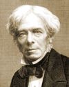 Michael
Faraday (1791-1867) was the son of a blacksmith,
and a bookbinder by trade...
In 1810, he started attending the lectures
that Humphry Davy (1778-1829) had been giving at
the Royal Institution of London since 1801.
In December 1811, Faraday became an assistant of Davy,
whom he would eventually surpass in knowledge and influence.
Faraday was elected to the Royal Society in 1824,
in spite of the jealous opposition of Sir Humphry
Davy who was its president (from 1820 to 1827).
Michael
Faraday (1791-1867) was the son of a blacksmith,
and a bookbinder by trade...
In 1810, he started attending the lectures
that Humphry Davy (1778-1829) had been giving at
the Royal Institution of London since 1801.
In December 1811, Faraday became an assistant of Davy,
whom he would eventually surpass in knowledge and influence.
Faraday was elected to the Royal Society in 1824,
in spite of the jealous opposition of Sir Humphry
Davy who was its president (from 1820 to 1827).
Arguably, the greatest of Faraday's many scientific contributions was
the Law of Induction which he formulated in 1831.
By explaining the 1821 observation of Oersted in terms of what
we now called the magnetic field, Faraday did much more than invent
the electric motor, he opened entirely new vistas for physics.
He proposed that light itself was an electromagnetic
phenomenon.
He lived to be proven right mathematically by his younger friend,
James Clerk Maxwell.
|
 |
| Heinrich Lenz |
Heinrich Lenz (1804-1865).
Lenz's Law (1833).
The magnetic flux...
F = B . S
dF =
dB . S +
B . dS
First term = Magnetic Induction. Second Term = Lorentz Force.
(2005-07-18) On the History of Maxwell's Equations
The basic laws of electricity and magnetism.
Gauss' Electric Law = Coulomb's Law
Gauss's Magnetic Law.
Faraday's Law of Induction.
Ampère's Law.
(2005-07-09) Maxwell's Equations Unify
Electricity and Magnetism
They predicted electromagnetic waves before Hertz demonstrated them.
Maxwell's equations govern the electromagnetic
quantities defined above :
- The electric field E
- The magnetic induction B
- The density of electric charge r
- The density of electric current j
Maxwell's Equations (1864)
| rot E + |
|
|
¶ B |
= 0 |
|
div E = |
r |
|
|
| ¶ t |
eo |
| rot B - |
1 |
¶ E |
= mo j |
div B = 0 |
|
|
| c2 |
¶ t |
|
The three electromagnetic constants involved are tied by one equation:
A direct consequence of Maxwell's equations is the following relation,
which expresses the conservation of electric charge
(HINT: div rot B vanishes...
The conclusion holds if and only if the 3
constants are related as advertised.)
Electric Charge is Conserved
| div j + |
¶ r |
= 0 |
|
| ¶ t |
|
Using the identity
rot rot V = grad div V - DV
when r = 0 and
j = 0, we obtain the following equality
for any electromagnetic component y.
| 1 | |
¶ 2 y |
= Dy |
|
|
| c 2 |
¶ t 2 |
This wave equation shows that the
electromagnetic field propagates at celerity c in a vacuum.
This led Maxwell to propose an electromagnetic theory of light.
The propagation of electromagnetic waves (radio waves) was
demonstrated experimentally in 1888, by Heinrich Rudolf
Hertz (1857-1894).
(2005-07-15)
Electromagnetic Planar Waves (Progressive Waves)
The simplest solutions to Maxwell's equations,
far from all sources.
In the absence of electromagnetic sources
( r = 0, j = 0 ) we may look for
electromagnetic fields whose values do not depend
on the y and z coordinates.
A solution of this type is called a
progressive planar wave and it's best established
directly from the above equations of Maxwell,
without resorting to the electromagnetic
potentials introduced below.
(2005-07-15)
Electromagnetic Energy & Poynting Vector
The Lorentz force transfers energy from the
field to the charge carriers.
The power F.v of the Lorentz force is
q E.v. Thus, the power received by the electric charges per unit of
volume is E.j.
The charge carriers may then convert the power so received from the local electromagnetic
field into other form of energy (including the kinetic energy of particles).
E.j may be expressed as follows,
in terms of the electromagnetic fields alone.
HINT:
Express j in terms of the fields with
Maxwell's equations, then use the
identity
E.rot B = B.rot E
- div E´B
and the relation rot E = -¶B/¶t
Electromagnetic Balance of Energy Density
(Poynting Theorem, 1884)
| div ( |
E ´ B |
) + |
¶ |
( |
eo E 2
+ B 2 / mo |
) =
- E . j |
|
|
|
| mo |
¶ t |
2 |
|
This relation is due to a former student of Maxwell,
John
Henry Poynting (1852-1914).
The vector S = E´B / mo is now called the Poynting vector.
The right-hand side of of the above equation is the opposite
of the power delivered by the field to the sources, per unit of volume.
It's therefore the density of the power released by the sources to the field.
The left-hand side is readily interpreted as evidence for
an energy carried by the electromagnetic field:
Electromagnetic Energy Density
|
|
In a given volume, this energy is either delivered directly by local sources or
it comes from radiation through its surface, as the flux of the Poynting vector.
(2005-07-13)
Electromagnetic Potentials & Lorenz Gauge
Devised by Ludwig Lorenz in 1867 [when H.A. Lorentz was only 14].
Since Maxwell's equations assert that
the divergence of B vanishes,
there is necessarily a vector potiental A
of which B is the rotational (or curl).
This implies that
rot [ E +
¶A/¶t ] = 0
which proves that the bracket is the gradient of a scalar potential, called
-f for compatibility with
electrostatics.
These two equations do not uniquely determine the potentials,
as the same fields are obtained with the following changes in the
potentials, for any scalar field y.
A ¬ A
+ grad y
f ¬ f - ¶y/¶t
This leeway can be used to make sure the following equation is satisfied,
as proposed by Ludwig Lorenz in 1867.
(Watch the spelling... There's no "t".)
The Lorenz Gauge (1867)
| div A + |
1 |
|
¶ f |
= 0 |
|
|
| c2 |
¶ t |
|
The Lorenz Gauge still allows the above type of leeway,
but only for an arbitrary field y
propagating freely at celerity c, according to the equation:
| 1 | |
¶ 2 y |
= Dy |
|
|
| c 2 |
¶ t 2 |
The two Maxwell equations which don't involve electromagnetic sources are equivalent to the
above definitions of E and B in terms of
electromagnetic potentials.
Using the Lorenz Gauge, the other two equations boil down to the following relations
between the electromagnetic sources and the potentials:
D'Alembert's Equations
| Df - |
1 |
|
¶ f |
= |
|
|
r |
|
|
|
|
| c2 |
¶ t |
|
eo |
| DA
- |
1 |
¶ A |
= - mo j |
|
|
| c2 |
¶ t |
|
Without the Lorenz Gauge, more complicated relations would hold:
| Df - |
1 |
|
¶ f |
= |
|
|
|
r |
|
|
|
¶ |
( div A + |
1 |
|
¶ f |
) |
|
|
|
|
|
|
|
|
| c2 |
¶ t |
|
eo |
|
¶ t |
c2 |
¶ t |
| DA
- |
1 |
¶ A |
= |
- mo j + grad |
( div A + |
1 |
|
¶ f |
) |
|
|
|
|
| c2 |
¶ t |
c2 |
¶ t |
Although it was once a mere mathematical convenience,
the Lorenz gauge is now considered fundamental,
because quantum theory assigns a physical
significance to electromagnetic potentials.
In particular, the following definition of the so-called
canonical momentum makes the Lorenz gauge mandatory:
Canonical momentum of a particle of
mass m, charge
q and velocity v|
|
The Aharonov-Bohm Effect
(2005-07-15)
Retarded and Advanced Potentials
General solutions of Maxwell's equations
obeying the Lorenz gauge.
As shown below,
the following potentials satisfy the Lorenz gauge
Electrodynamic Retarded Potentials A-
and f-
| f-(t,r) |
= |
òòò |
r ( t - ||r-s|| / c , s ) |
d3s |
|
| 4peo
|| r - s || |
| A-(t,r) |
= |
òòò |
mo j ( t - ||r-s|| / c , s ) |
d3s |
|
| 4p
|| r - s || |
|
This is similar to the expressions obtained in the static cases
(electrostatics, magnetostatics) except
that the fields we observe here and now
depend on a prior state of the sources.
The influence of the sources is delayed by the time it would
take the "news" of their changing state to travel at speed c.
There's also another solution
(the so-called advanced potentials
A+ and f+ )
which is formally obtained from the above by changing the sign of c,
or equivalently by reversing the
arrow of time.
This is just like what we've already encountered
in the case of planar waves,
with two possible directions of travel.
However, the physical interpretation is not nearly as easy now that we're
dealing with some causality relationship between the field and its
"sources".
Advanced potentials make the situation here and now
(potentials and/or fields) depend on the future
state of remote "sources".
Such a thing may be summarily dismissed as "unphysical" but this fails
to make the issue go away.
Indeed, quantum treatments of electromagnetic fields (photons in
Quantum Field Theory )
imply that a field can create some of its sources in the form of charged
particle-antiparticle pairs.
What seems to be lacking is the coherence
of such creations because of statistical and/or thermodynamical
considerations (which feature a pronounced arrow of time).
I don't understand this. Nobody does...
What's clear, however, is that the distinction between past and future vanishes
in stationary cases.
This makes advanced potentials relevant and/or necessary,
without the need for mind-boggling philosophical considerations.
Here's the outline of a proof that the
retarded potentials satisfy the
Lorenz gauge, as advertised... (The same is true of the advanced potentials.)
Consider the integrands for a fixed position of the source
(that's what s is).
(2005-08-21)
Electrodynamic Fields
A general expression derived from the above retarded potentials.
Letting R be
|| r - s ||
the retarded potentials yield the following fields, where
r and j stand, respectively, for
r ( t - R / c
, s ) and
j ( t - R / c , s ).